
PromQL is superb for metrics alerting and graphing needs, for heavier statistical work there are better options.
R is one of the standard pieces of software for doing statistics, with many libraries available for it. I'm not going to go into great depth into R itself, as that's a very big topic but just give you a taste of what's possible. I'm going to presume you already have R installed (it's r-base for Debian-based users, and R for those using Homebrew).
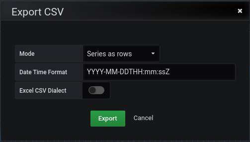
Go to Grafana and on a graph panel click the triangle just to the right of the panel title, hover over More... on the menu that pops up, and then click Export CSV. You can then Export from the dialog that appears:
You can now start R, read this data and parse the timestamp:
> dat = read.csv("grafana_data_export.csv", header = TRUE, ";", na.strings=c("null"))
> data = data.frame(dat, ts=xtfrm(as.POSIXct(dat$Time,format="%Y-%m-%dT%H:%M:%S")))
> head(data)
  Series                      Time  Value         ts
1 Chunks 2019-09-24T12:00:00+00:00  92758 1569322800
2 Chunks 2019-09-24T13:00:00+00:00 139141 1569326400
3 Chunks 2019-09-24T14:00:00+00:00  88662 1569330000
4 Chunks 2019-09-24T15:00:00+00:00 137093 1569333600
5 Chunks 2019-09-24T16:00:00+00:00  92758 1569337200
6 Chunks 2019-09-24T17:00:00+00:00 141189 1569340800
If you suspected that this metric was going up over time you could do a linear regression trying to explain the Value by ts:
> summary(lm(Value~ts, data))

Call:
lm(formula = Value ~ ts, data = data)

Residuals:
   Min     1Q Median     3Q    Max
-27562 -24022 -21258  24474  27582

Coefficients:
              Estimate Std. Error t value Pr(>|t|)
(Intercept) -4.603e+06  5.927e+06  -0.777    0.438
ts           3.007e-03  3.775e-03   0.797    0.426


Residual standard error: 24270 on 335 degrees of freedom
Multiple R-squared: 0.001891, Adjusted R-squared: -0.001089
F-statistic: 0.6346 on 1 and 335 DF, p-value: 0.4262
This is the same math that deriv/predict_linear do however R also helps you determine if the analysis makes sense. In this case the ts isn't significant, so it's probably not going up over time.
However this particular metric is about Prometheus itself, and is related to the 2h compaction cycle, so you could take that info account:
> summary(lm(Value~ts+ts%%7200, data))

Call:
lm(formula = Value ~ ts + ts%%7200, data = data)

Residuals:
    Min      1Q  Median      3Q     Max
-6654.6  -786.1   173.8  1126.0  3368.9

Coefficients:
              Estimate Std. Error t value Pr(>|t|)
(Intercept) -4.579e+06  4.074e+05  -11.24   <2e-16 ***
ts           3.007e-03  2.595e-04   11.59   <2e-16 ***
ts%%7200    -1.341e+01  5.049e-02 -265.66   <2e-16 ***
---
Signif. codes:  0 ‘***’ 0.001 ‘**’ 0.01 ‘*’ 0.05 ‘.’ 0.1 ‘ ’ 1

Residual standard error: 1668 on 334 degrees of freedom
Multiple R-squared:  0.9953,    Adjusted R-squared:  0.9953
F-statistic: 3.535e+04 on 2 and 334 DF,  p-value: < 2.2e-16
This looks more promising as there's significant effects, and the correlation coefficient R-squared is close to 1.0. From the line
ts 3.007e-03 2.595e-04 11.59 <2e-16 ***
it would seem that the value is going up by about .003 per second. So we could graph this regression line ignoring the last coefficient:
> c = lm(Value~ts+ts%%7200, data)$coefficients
> plot(data$Value ~ data$ts)
> lines(data$ts, c[1] + c[2]*data$ts, col='red', lwd=3)
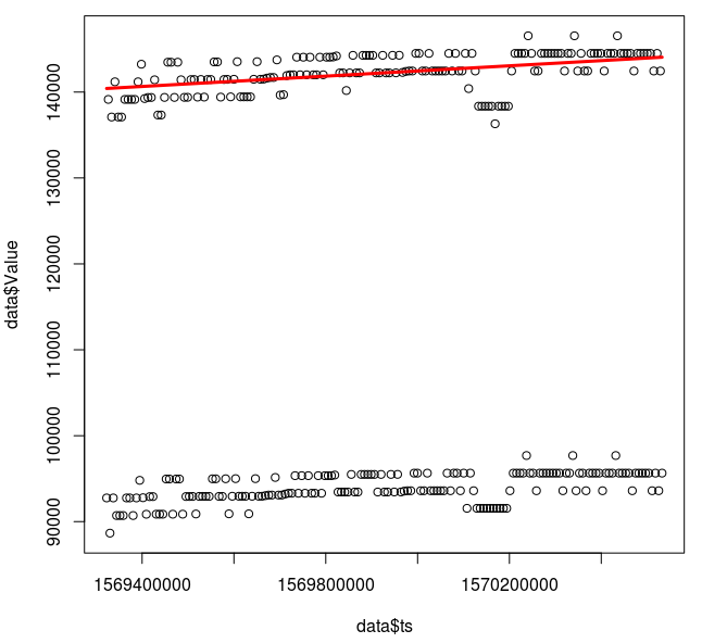
This looks like a good fit, though it'd be wise to check that outliers aren't overly impacting the result and that the relationship is actually linear.
This is a small glimpse of what's possible with R. For more serious work you might export data from Prometheus directly, use an ANOVA to determine what variables matter, perform predictions, and use packages like the one for Universal Scalability Law when doing capacity planning.
Want to get the most out of your metrics? Contact us.


No comments.